The scio package generates AI-powered summaries of R objects (e.g., data frames, plots, text) via the OpenRouter API. It was originally intended as a tool to streamline the summarization of outputs during iterative analyses in R notebooks.
Setup
Initialize scio and configure the environment for the examples below.
# Configure chunk options
knitr::opts_chunk$set(
  collapse = TRUE,
  comment  = "#>"
)

# Load package
library(scio)
# Sys.setenv(OPENROUTER_API_KEY = "<your_key>")

# Check if API key is available
CAN_RUN <- nzchar(Sys.getenv("OPENROUTER_API_KEY"))
PLACEHOLDER <- "*(API call skipped: OPENROUTER_API_KEY not set)*"

# Wrapper function for clean output
summary_output <- function(x) {
  if (CAN_RUN) {
    knitr::asis_output(paste("**Summary:**", get_summary(x)))
  } else {
    PLACEHOLDER
  }
}
Alternatively, set your
OPENROUTER_API_KEYin your .Renviron file.
Summarizing Text
Generate summaries from text strings.
analysis_intro <- "
We are conducting a comprehensive analysis of the mtcars dataset to understand
the relationship between vehicle weight and fuel efficiency, with implications
for automotive design decisions.
"
summary_output(analysis_intro)
Summary: The analysis focuses on the relationship between vehicle weight and fuel efficiency in the mtcars dataset. It aims to identify patterns that could influence automotive design decisions.
Summarizing Data Frames
Work with data frames and their summary outputs.
df_summary <- summary(mtcars)
df_summary
#>       mpg             cyl             disp             hp
#>  Min.   :10.40   Min.   :4.000   Min.   : 71.1   Min.   : 52.0
#>  1st Qu.:15.43   1st Qu.:4.000   1st Qu.:120.8   1st Qu.: 96.5
#>  Median :19.20   Median :6.000   Median :196.3   Median :123.0
#>  Mean   :20.09   Mean   :6.188   Mean   :230.7   Mean   :146.7
#>  3rd Qu.:22.80   3rd Qu.:8.000   3rd Qu.:326.0   3rd Qu.:180.0
#>  Max.   :33.90   Max.   :8.000   Max.   :472.0   Max.   :335.0
#>       drat             wt             qsec             vs
#>  Min.   :2.760   Min.   :1.513   Min.   :14.50   Min.   :0.0000
#>  1st Qu.:3.080   1st Qu.:2.581   1st Qu.:16.89   1st Qu.:0.0000
#>  Median :3.695   Median :3.325   Median :17.71   Median :0.0000
#>  Mean   :3.597   Mean   :3.217   Mean   :17.85   Mean   :0.4375
#>  3rd Qu.:3.920   3rd Qu.:3.610   3rd Qu.:18.90   3rd Qu.:1.0000
#>  Max.   :4.930   Max.   :5.424   Max.   :22.90   Max.   :1.0000
#>        am              gear            carb
#>  Min.   :0.0000   Min.   :3.000   Min.   :1.000
#>  1st Qu.:0.0000   1st Qu.:3.000   1st Qu.:2.000
#>  Median :0.0000   Median :4.000   Median :2.000
#>  Mean   :0.4062   Mean   :3.688   Mean   :2.812
#>  3rd Qu.:1.0000   3rd Qu.:4.000   3rd Qu.:4.000
#>  Max.   :1.0000   Max.   :5.000   Max.   :8.000
summary_output(df_summary)
Summary: Miles per gallon (mpg) ranges from 10.4 to 33.9 with a mean of 20.09, while horsepower (hp) varies from 52 to 335 with a mean of 146.7. The number of cylinders (cyl) mostly clusters around 4, 6, and 8, with a mean of 6.188, and weight (wt) spans from 1.513 to 5.424 with an average of 3.217. Transmission type (am) has a mean of 0.4062 indicating fewer manual transmissions, and gear counts range from 3 to 5 with a mean of 3.688.
Summarizing Plots
Create summaries from ggplot objects.
library(ggplot2)
plot_cars <- ggplot(mtcars, aes(mpg, wt)) +
  geom_point() +
  geom_smooth(method = "lm") +
  labs(
    title = "Vehicle Weight vs Fuel Efficiency",
    x = "Miles per Gallon (MPG)",
    y = "Weight (1000 lbs)")
plot_cars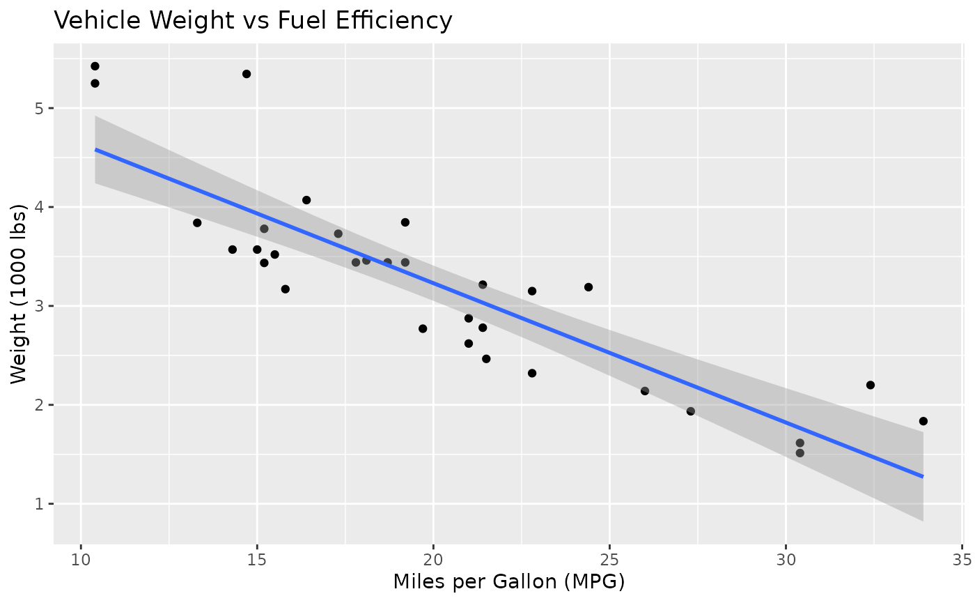
summary_output(plot_cars)Summary: Vehicle data shows that cars with higher miles per gallon (mpg) generally have lower weight (wt), with mpg ranging from 10.4 to 33.9 and weight from 1.513 to 5.424 (1000 lbs). The dataset includes various car models with differing cylinder counts, horsepower, and transmission types, illustrating a negative relationship between vehicle weight and fuel efficiency.
Summarizing Statistical Models
Handle model objects and their outputs.
linear_model <- lm(mpg ~ wt, data = mtcars)
summary(linear_model)
#>
#> Call:
#> lm(formula = mpg ~ wt, data = mtcars)
#>
#> Residuals:
#>     Min      1Q  Median      3Q     Max
#> -4.5432 -2.3647 -0.1252  1.4096  6.8727
#>
#> Coefficients:
#>             Estimate Std. Error t value Pr(>|t|)
#> (Intercept)  37.2851     1.8776  19.858  < 2e-16 ***
#> wt           -5.3445     0.5591  -9.559 1.29e-10 ***
#> ---
#> Signif. codes:  0 '***' 0.001 '**' 0.01 '*' 0.05 '.' 0.1 ' ' 1
#>
#> Residual standard error: 3.046 on 30 degrees of freedom
#> Multiple R-squared:  0.7528, Adjusted R-squared:  0.7446
#> F-statistic: 91.38 on 1 and 30 DF,  p-value: 1.294e-10
summary_output(linear_model)
Summary: The data shows a linear regression model of miles per gallon (mpg) predicted by weight (wt) for various car models, with an intercept around 37.29 and a negative coefficient for weight (-5.34), indicating mpg decreases as weight increases. Individual car coefficients vary, with lighter cars like Honda Civic and Toyota Corolla having positive residuals and heavier cars like Cadillac Fleetwood and Lincoln Continental showing large negative residuals. The dataset includes mpg and weight values for 32 car models, reflecting a general inverse relationship between weight and fuel efficiency.
Summarizing Multiple Objects
Process a list of objects to create combined
summaries.
report_summary <- get_summary(list(
  analysis_intro,
  df_summary,
  linear_model,
  plot_cars
  ))
#> `geom_smooth()` using formula = 'y ~ x'
With the default
aggregate_list = TRUE, it will create an integrated summary based on all items in the list. This is useful for summarizing related pieces of information together (e.g., dataset excerpt, statistical model, and accompanying plot).
Inline Summaries
For automated reports or inline documentation, embed summaries directly.
To embed report_summary directly in text, place
`r report_summary` here, which produces:
Vehicle weight negatively correlates with fuel efficiency, with each 1000 lb increase in weight associated with a decrease of approximately 5.344 MPG. The data shows a clear downward trend in weight as miles per gallon increase, supported by a linear regression model with an intercept of 37.285.
Configuration
Customize behavior using environment variables.
Sys.setenv(
  OPENROUTER_MODEL       = "meta-llama/llama-4-maverick:free",
  OPENROUTER_TOKEN_LIMIT = "250"
)
Customizing Prompts
Modify AI prompts to change summary style and focus.
Sys.setenv(
  OPENROUTER_SYSTEM_MESSAGE =
    "You are a data science expert summarizing R outputs.",
  OPENROUTER_INSTRUCTION =
    "Provide a brief 2-3 sentence interpretation focusing on key patterns."
)
After setting these, scio will use them on the next
summary_output() call:
summary_output(report_summary)Summary: Vehicle weight is inversely related to fuel efficiency, with each 1000 lb increase resulting in about a 5.344 MPG decrease. The linear regression model indicates a starting fuel efficiency of 37.285 MPG when weight is zero, confirming a downward trend in weight as miles per gallon increase.
Troubleshooting
- Ensure
OPENROUTER_API_KEYis set. - Check your internet connection.
- For more information, see the package GitHub page.